Another worked example
|
|
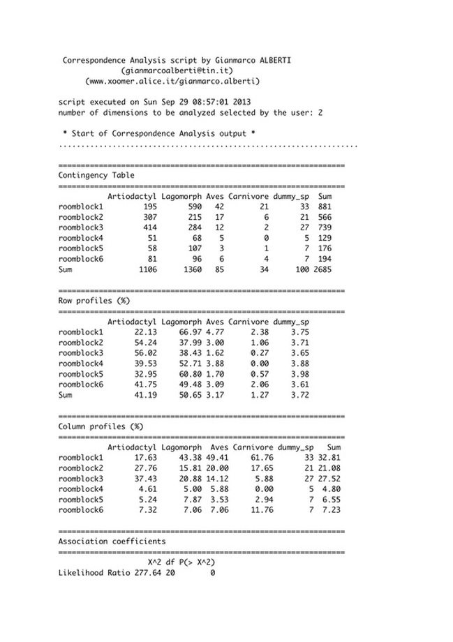
For illustrative purposes, we take into account a dataset derived from the article by James M. Potter, Communal Ritual and Faunal Remains: An Example from the Dolores Anasazi, Journal of Field Archaeology, 24(3), 1997, 354-64. The dataset can be found on page 360 (Table 2). It reports the number of identifiable specimens of 4 major taxonomic groups for each roomblock within the Puebloan McPhee Village (in the US Four Corners region). The author wished to address the expectation concerning the abundance of certain taxonomic orders across the site. In other words, for the sake of any subsequent anthropological/archaeological interpretation of the patterns of utilization of different animal species, the analyst was interested in exploring the degree to which different faunal remains "correspond" to different sector of the village.
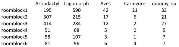
The dataset (available HERE) is reproduced here, with two slight modifications: (i) the original name of the roomblocks have been sustituted with simpler labels (roomblock 1, 2, etc.); (ii) a fifth category (corresponding to the average colum profile and labelled dummy_sp[ecie]) has been added just for illustrative purposes, to make evident what a profile similar to the average one will look like in the CA scatterplot.
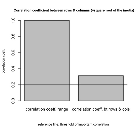
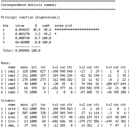
The dependency between rows and columns can be considered important (i.e., strong), since it is above the 0.2 threshold (actually, 0.314). See the chart below. Further, the chi-square statistic is equal to 265.42 (df 20), which is highly significant (well below alpha 0.01).
CA allows to isolate one main dimension of variability in the data. In fact, one out of the 4 dimensions turns out to account for the majority of the inertia (actually, 95.9%).
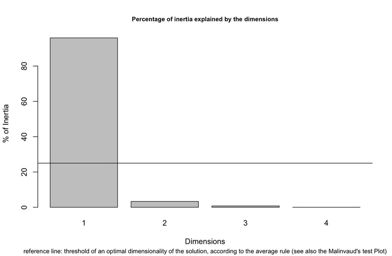
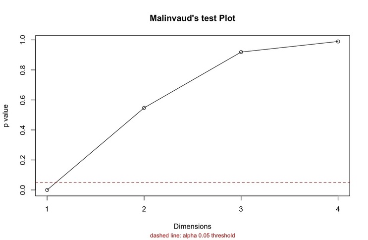
The 1 dimension is the only one that appears to be significant according to the scree plot, the so-called average rule and the Malinvaud's Test (all discussed earlier in this site). The chart related to the latter test is shown below.
Since we are interested in understanding the similarities between roomblock as far as faunal species remains are concerned, it could be decided to interpret the position of the roomblocks in the sub-space defined by the faunal species (i.e., column categories).
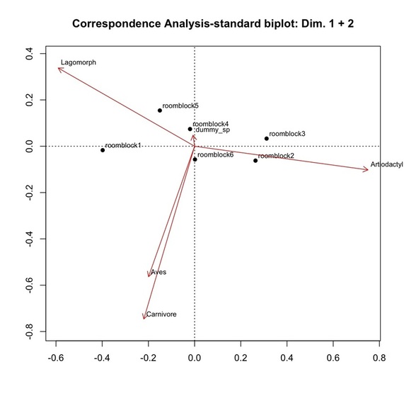
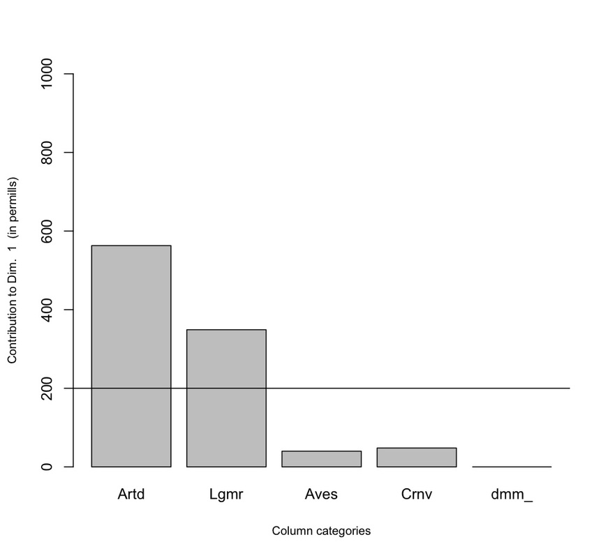
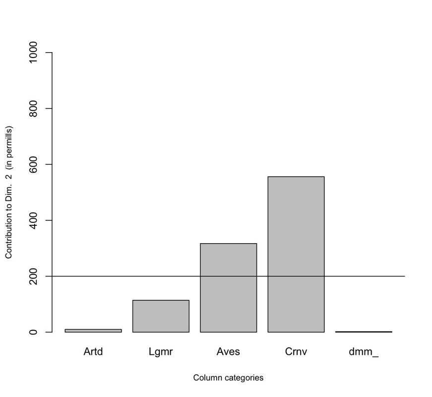
As shown below (left) by the Standard Biplot (discussed earlier in this site), the opposite poles of the (dominant and significant) first dimension are determined by two species: Lagomorph (negative pole), Artiodactyl (positive pole). The second dimension is determined by Aves and Carnivore. The same information can be also derived from the two bar plots further below, which dysplay the contribution (in permills) of faunal species to the first two dimensions, with the reference line indicating the threshold above which a contribution can be considered worth considering. Incidentally, it must be noted that the contribution of the dummy species is practically nihil: since it corresponds to the average colum profile, it does not contribute in differenziating between roomblock's assemblages.
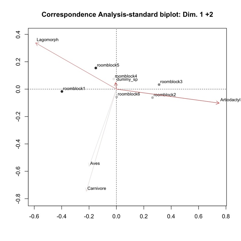
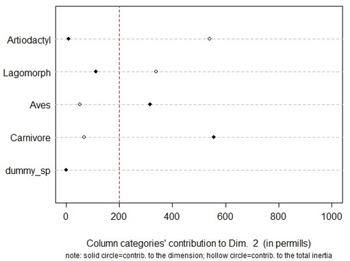
It must be kept in mind, however, that the second dimension accounts for a very low proportion of the total inertia (actually, 3.3%). This can be appreciated by inspecting: a) the Standard Biplot (below, right); b) the dot chart provided by my 'CAinterprTools' described in this same site (see figure further below). In the former, the vectors representing the species (i.e., column categories) have colour intensity proportional to their absolute contribution to the total inertia. It can be seen that, while Aves and Carnivore have a high contribution to the definition of the second dimension (proportional to the lenght of the vector), they have a low contribution to the inertia (i.e., variability) of the table overall (proportional to the colour intensity, as said). The dot chart provided by my 'CAinterprTools' package allows to appreciate in a very straightforward way that the two mentioned species have an important contribution to the definition of the 2 dimension (solid circle) while they are poorly contributing to the total inertia of the data (hollow circle).
As shown below (left) by the Standard Biplot (discussed earlier in this site), the opposite poles of the (dominant and significant) first dimension are determined by two species: Lagomorph (negative pole), Artiodactyl (positive pole). The second dimension is determined by Aves and Carnivore. The same information can be also derived from the two bar plots further below, which dysplay the contribution (in permills) of faunal species to the first two dimensions, with the reference line indicating the threshold above which a contribution can be considered worth considering. Incidentally, it must be noted that the contribution of the dummy species is practically nihil: since it corresponds to the average colum profile, it does not contribute in differenziating between roomblock's assemblages.
It must be kept in mind, however, that the second dimension accounts for a very low proportion of the total inertia (actually, 3.3%). This can be appreciated by inspecting: a) the Standard Biplot (below, right); b) the dot chart provided by my 'CAinterprTools' described in this same site (see figure further below). In the former, the vectors representing the species (i.e., column categories) have colour intensity proportional to their absolute contribution to the total inertia. It can be seen that, while Aves and Carnivore have a high contribution to the definition of the second dimension (proportional to the lenght of the vector), they have a low contribution to the inertia (i.e., variability) of the table overall (proportional to the colour intensity, as said). The dot chart provided by my 'CAinterprTools' package allows to appreciate in a very straightforward way that the two mentioned species have an important contribution to the definition of the 2 dimension (solid circle) while they are poorly contributing to the total inertia of the data (hollow circle).
|
|
|
The latter point can be further appreciated by inspecting a section of the Script's textual output (after the 'ca' package).
It can be easily seen that while Aves and Carnivore have a high contribution (ctr) to the definition of the second dimension (k2) (317 and 556 in permills respectively, equals to 31.7% and 55.6%), resulting in a considerable lenght of their vectors in the Standard Biplot, their contribution to the overall inertia (inr) is low (53 and 68 in permills, equal to 5.3% and 6.8%), resulting in a low colour intensity of their vectors. |
|
|
|
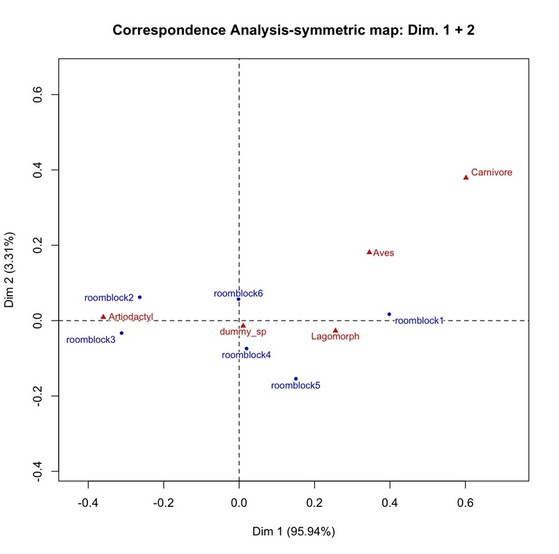
The CA scatterplot is shown to the left.
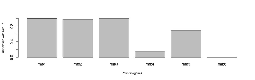
It is apparent that the main difference in faunal species CA is helping to pinpointing is that between Artiodactyl and Lagomorph. On this respect, roomblocks 2 and 3 (having the highest proportion of the first specie) are opposed to 1 and 5 (where the second specie dominates). Needless to say, these roomblocks are highly correlated with the first dimension (see bar plot below). The fact that roomblocks 4 and 6 are positioned near the centre of the plot (relative to the first dimension) means that they are little differentiated as far as those two species are concerned; in other words, the distribution of those species in those roomblocks does not dramatically depart from the average. The second (vertical) dimension, determined by Aves and Carnivore, barely opposes roomblocks 6 to the others, meaning that the former has an higher propotion of those species. It must be keept in mind, however, that the difference seems negligible since, as noted, the second dimensions accounts for a very tiny portion of the total inertia. |
|
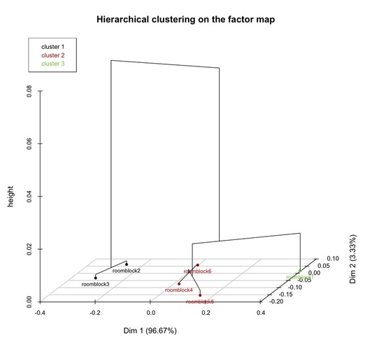
Finally, rows clustering (discussed earlier in this site) indicated that a two-clusters solution seems sound, with roomblocks 2 and 3 apposed to a larger cluster made up of roomblocks 1, 4, 5, and 6.
Roomblock 1 stands further apart since, as seen, it is the one having the highest proportion of Lagomorph. It has be noted that in this analysis roomblock 5 appears to be more similar to 4 and 6. It should not surprise since, unlike roomblock 1, 5 is correlated to the second dimension as well. |
Below, you can see the first page of the textual report provided by my R script for CA, which you can find at this page of this site. The full report can be downloaded from this link.
Finally, for the illustration of this worked example in the context of the description of an additional R Script for CA, see this page of this site.
Finally, for the illustration of this worked example in the context of the description of an additional R Script for CA, see this page of this site.
Have you found this website helpful? Consider to leave a comment in this page.
