'auc.adjust': R function for optimism-adjusted AUC (internal validation) (DOI: 10.13140/RG.2.1.1485.0324)
'auc.adjust' is an R function which allows to calculate the AUC of a (binary) Logistic Regression model, adjusted for optimism. In essence, the function performs an internal validation of a model via a bootstrap procedure (devised by Harrell et al) , which enable to estimate the degree of optimism of a fitted model and the extent to which the model will be able to generalize outside the training dataset. If you want more info, you can refer to this website (LINK), and/or read the following interesting article (in which the bootstrap procedure is described at page 776):
Steyerberg, E. W., Harrell, F. E., Borsboom, G. J. J. ., Eijkemans, M. J. ., Vergouwe, Y., & Habbema, J. D. F. (2001). Internal validation of predictive models. Journal of Clinical Epidemiology, 54(8), 774–781. http://doi.org/10.1016/S0895-4356(01)00341-9
The function is quite straightforward:
auc.adjust(data, fit, B)
where:
data is a dataframe containing your dataset (note: the Dependent Variable must be stored in the first column to the left),
fit is the object returned from glm() function,
B is the desired number of bootstrap resamples (suggested values: 100 or 200).
Before focusing on the outcome of the function, let's see it in action by means of an example.
First, let's create a fictional dataset with 1 binary DV, 2 continuous and 1 categorical Predictors (I took this dataset from this website -> LINK):
mydata <- read.csv("http://www.ats.ucla.edu/stat/data/binary.csv")
mydata$rank <- factor(mydata$rank)
Once we got our dataset, let's fit a Logistic Regression model, storing it in an object named 'model':
model <- glm(admit ~ gre + gpa + rank, data = mydata, family = "binomial")
Once we have the data and the fitted model, putting the function at work is very easy:
auc.adjust(mydata, model, B=200)
The function may take a while to run, it depends on the size of your dataset and on the number of bootstrap resamples.
The following plot is returned:
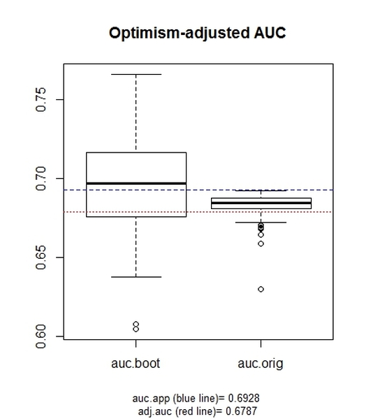
The boxplots represent:
-the distribution of the AUC value in the bootstrap sample (auc.boot), which represents "an estimation of the apparent performance" (according to the aforementioned reference);
-the distribution of the AUC value deriving from the model fitted to the bootstrap samples and evaluated on the original sample (auc.orig), which represents the model performance on independent data.
At the bottom of the chart, the apparent AUC (i.e., the value deriving from the model fitted to the original dataset) and the AUC adjusted for optimism are reported.
For an example of the use and interpretation of the optimism-adjusted AUC, see for example:
Faraklas I, Stoddard GJ, Neumayer L a., Cochran A. Development and validation of a necrotizing soft-tissue infection mortality risk calculator using nsqip. J Am Coll Surg. 2013;217: 153–160.e3. doi:10.1016/j.jamcollsurg.2013.02.029
The function's code is reported below (or you can download it from this LINK). You can copy/paste it straight into R. Note that, in order for the function to work, the 'pROC' and 'kimisc' packages must be already installed and loaded into R.
auc.adjust <- function(data, fit, B){
fit.model <- fit
data$pred.prob <- fitted(fit.model)
auc.app <- roc(data[,1], data$pred.prob, data=data)$auc # require 'pROC'
auc.boot <- vector (mode = "numeric", length = B)
auc.orig <- vector (mode = "numeric", length = B)
o <- vector (mode = "numeric", length = B)
for(i in 1:B){
boot.sample <- sample.rows(data, nrow(data), replace=TRUE) # require 'kimisc'
fit.boot <- glm(formula(fit.model), data = boot.sample, family = "binomial")
boot.sample$pred.prob <- fitted(fit.boot)
auc.boot[i] <- roc(boot.sample[,1], boot.sample$pred.prob, data=boot.sample)$auc
data$pred.prob.back <- predict.glm(fit.boot, newdata=data, type="response")
auc.orig[i] <- roc(data[,1], data$pred.prob.back, data=data)$auc
o[i] <- auc.boot[i] - auc.orig[i]
}
auc.adj <- auc.app - (sum(o)/B)
boxplot(auc.boot, auc.orig, names=c("auc.boot", "auc.orig"))
title(main=paste("Optimism-adjusted AUC", "\nn of bootstrap resamples:", B), sub=paste("auc.app (blue line)=", round(auc.app, digits=4),"\nadj.auc (red line)=", round(auc.adj, digits=4)), cex.sub=0.8)
abline(h=auc.app, col="blue", lty=2)
abline(h=auc.adj, col="red", lty=3)
}
Have you found this website helpful? Consider to leave a comment in this page.
