'model.valid': R function for binary Logistic Regression internal validation (DOI: 10.13140/RG.2.1.1925.6086)
'model.valid' is an R function which allows perform internal validation of a binary Logistic Regression model, implementing part of the procedure described by:
Arboretti Giancristofaro R, Salmaso L. Model performance analysis and model validation in logistic regression. Statistica 2003(63): 375–396.
The procedure consists of the following steps:
1) the whole dataset is split into two random parts, a fitting (75%) and a validation (25%) portion;
2) the model is fitted on the fitting portion (i.e., its coefficients are computed considering only the observations in that portion) and its performance is evaluated on both the fitting and the validation portion, using AUC as performance measure;
3) steps 1-2 are repeated B times, eventually getting a fitting and validation distribution of the AUC values. The former provides an estimate of the performance of the model in the population of all the theoretical training samples; the latter represents an estimate of the model’s performance on new and independent data.
The function is quite straightforward:
model.valid(data, fit, B)
where:
data is a dataframe containing your dataset (note: the Dependent Variable must be stored in the first column to the left),
fit is the object returned from glm() function,
B is the desired number of iterations (see description of the procedure above).
Before focusing on the outcome of the function, let's see it in action by means of an example.
First, let's create a fictional dataset with 1 binary DV, 2 continuous and 1 categorical Predictors (I took this dataset from this website -> LINK):
mydata <- read.csv("http://www.ats.ucla.edu/stat/data/binary.csv")
mydata$rank <- factor(mydata$rank)
Once we got our dataset, let's fit a binary Logistic Regression model, storing it in an object named 'model':
model <- glm(admit ~ gre + gpa + rank, data = mydata, family = "binomial")
Once we have the data and the fitted model, putting the function at work is very easy:
model.valid(mydata, model, B=1000)
The function may take a while to run, it depends on the size of your dataset and on the size of B.
The following plot is returned:
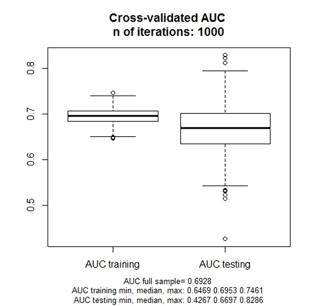
The chart represents the training and the testing (i.e., validation) distribution of the AUC value across the 1000 iterations.
For an example of the interpretation of the chart, see the aforementioned article, especially page 390-91.
The function's code is reported below (or you can download it from this LINK). You can copy/paste it straight into R. Note that, in order for the function to work, the 'pROC' and 'caTools' packages must be already installed and loaded into R.
model.valid <- function(data,fit,B){
auc.train <- vector(mode = "numeric", length = B)
auc.test <- vector(mode = "numeric", length = B)
data$pred.prob.full <- fitted(fit)
auc.full <- roc(data[,1], data$pred.prob.full, data=data)$auc
for(i in 1:B){
sample <- sample.split(data[,1], SplitRatio = .75) #require caTools
train <- subset(data, sample == TRUE)
test <- subset(data, sample == FALSE)
fit.train <- glm(formula(fit), data = train, family = "binomial")
train$pred.prob <- fitted(fit.train)
auc.train[i] <- roc(train[,1], train$pred.prob, data=train)$auc #require pROC
test$pred.prob.back <- predict.glm(fit.train, newdata=test, type="response")
auc.test[i] <- roc(test[,1], test$pred.prob.back, data=test)$auc
}
auc.train.min <- round(min(auc.train), digits=4)
auc.train.max <- round(max(auc.train), digits=4)
auc.train.median <- round(median(auc.train), digits=4)
auc.test.min <- round(min(auc.test), digits=4)
auc.test.max <- round(max(auc.test), digits=4)
auc.test.median <- round(median(auc.test), digits=4)
boxplot(auc.train, auc.test, names=c("AUC training", "AUC testing"))
title(main=paste("Cross-validated AUC", "\nn of iterations:", B), sub=paste("AUC full sample=", round(auc.full, digits=4), "\nAUC training min, median, max:", auc.train.min, auc.train.median, auc.train.max, "\nAUC testing min, median, max:", auc.test.min, auc.test.median, auc.test.max), cex.sub=0.8)
}
Have you found this website helpful? Consider to leave a comment in this page.
