Number of dimensions useful for data interpretation
|
|
It has to be stressed that this is one of the “thorniest” problem (Preacher et al. 2013, 29) affecting CA as well as Factor Analysis, Principal Components Analysis (PCA) and Multidimensional Scaling (see, e.g., Jackson 1993; Wilson, Cooper 2008; Van Pool, Leonard 2011, 296-299). As stressed by Hair et al. (2009, 591), in selecting the optimal number of dimensions the analyst is faced with the need of a trade-off between the increasing explained data variability deriving by keeping many dimensions versus the increasing complexity that can make difficult the interpretation of more than two dimensions. Like for other techniques, for which a number of approaches exists each having its pros and cons (overviews in Worthington, Whittaker 2006, 820-822; Wilson, Cooper 2008), also in CA there is no clear-cut rule guiding the analyst’s choice (Lorenzo-Seva 2011, 97) and different approaches have been proposed.
A more informal approach leans toward considering the number of useful dimensions fixed by the very analyst’s ability to give meaningful interpretation of the retained axes (Benzécri 1992, 398; Blasius, Greenacre 1998, 25; Yelland 2010, 13). In other words, dimensions that cannot be sensibly interpreted can be considered the result of random fluctuations among the residuals (Clausen 1998, 25).
Another approach would be to keep as many dimensions as necessary to account for the majority of the total inertia, setting a cut-off threshold at an arbitrary level, say 90% (see, in the context of Factor Analysis, Van Pool, Leonard 2011, 296). On the other hand, Hair et al. (2009, 591) suggest that dimensions whose inertia is greater than 0.2 (in terms of eigenvalue) should be included in the analysis.
Another frequently used method is the inspection of the scree plot, adapted from the context of PCA (Cattell 1966). Dimensions are plotted in order of the decreasing amount of explained inertia, resulting in a falling curve. The point at which the latter shows a bend (so called “elbow”) can be considered as indicating an optimal dimensionality (e.g., Clausen 1998, 24; Drennan 2009, 286-288; Van Pool, Leonard 2011, 296-297). It is worthy of note that this method has been found to perform fairly well (Zwick, Velicer 1986, 440; Bandalos, Boehm-Kaufman 2009, 81; Lorenzo-Seva 2011, 97).
The average rule, as termed by Lorenzo-Seva (2011, 97), is yet another method, which is equivalent to the Kaiser’s rule in the context of PCA (Wilson, Cooper 2008, with references). According to this rule, analysts should retain all the dimensions that explain more than the average inertia (expressed in terms of percentages), the latter being equal to 100 divided by the number of dimensions (i.e., the number of rows or columns, whichever is smaller, minus 1). Unfortunately, in the context of PCA, this method seems to overestimate the dimensionality of the solution (Wilson, Cooper 2008, 866; Lorenzo-Seva 2011, 97).
Saporta (2006, 209-210) has suggested the use of the Malinvaud’s test as guidance for the dimensionality of the CA solution (see also Camiz, Gomes 2013, 12). In practice, referring to Saporta’s book or Camiz-Gomez’s article for the computational details (see also Rakotomalala 2013, 7), this sequential test checks the significance of the remaining dimensions once the first k ones have been selected. Unfortunately, as stressed by Saporta himself and empirically tested by Rakotomalala (2013), it seems tends to overestimate the number of dimensions as the table’s grand total increases.
Finally, Lorenzo-Seva (2011) has interestingly adapted to CA a method developed for PCA, called Parallel Analysis. Its rationale is that nontrivial dimensions should explain a larger percentage of inertia than the dimensions derived from random data (update 2017: see the sig.dim.perm.scree() function implemented in the CAinterprTools package described at this page in this same site). While this method outperforms the aforementioned average rule, it seems to suggest a dimensionality of the solution comparable to the one that can be derived from the scree plot, at least in the illustrative example discussed by the scholar (Lorenzo-Seva 2011, 101, fig. 1).
In front of the sizable number of different approaches, each one having its pros and cons, I would lean toward a middle ground as to the problem of the dimensionality of the CA solution, trying to conciliate formal testing, on the one hand, with conceptual interpretability as dimension-retention criterion, on the other hand. I would agree with Worthington, Whittaker (2006, 822) who lucidly state that “in the end, researchers should retain a factor only if they can interpret it in a meaningful way no matter how solid the evidence for its retention”. In their opinion, exploratory approaches are “ultimately a combination of empirical and subjective approaches to data analysis because the job in not complete until the solution makes sense”. Within this general framework, I would also agree with Bandalos, Boehm-Kaufman (2009, 80-81) as to the need to compare and find a balance between different methods, provided that one deals always with significant factors according to the chi-square statistic.
The methods provided by the script are the average rule, the scree plot, and the Malinvaud’s test. A fourth criterion, namely the retention of dimensions whose eigenvalue is greater than 0.2 (sensu Hair et al. 2009 previously quoted), can be easily put to work thanks to the script output (via the ‘ca’ package), as will be described shortly. The reason for the choice of these methods rests on their wide use in literature, the good performance of the second (even compared to the aforementioned Parallel Analysis), and the opportunity to provide the users with the possibility to compare at least four of the criterions previously illustrated.
As for the average rule in the context of our worked example, any axis contributing more than the average percentage of inertia (100/11=9% in terms of rows, 100/6=16.7% in term of columns) should be considered important for the interpretation of the data (see, e.g., Bendixen 1995, 577). It must be acknowledged, however, that interesting patterns can emerge by inspecting more than just the first two dimensions, as rightly stressed by Baxter (1994, 120). With this warning in mind, the bar chart provided by the script can be used as a guidance in the choice of the relevant dimensions.
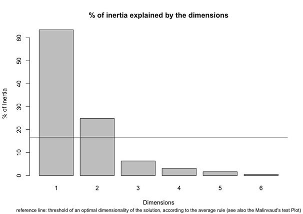
Dimensions are plotted in order of the decreasing amount of explained inertia. A reference line represents the threshold above which a dimension can be considered important according to the average rule. In our case, a 2-dimensional solution seems appropriate, with the first explaining over 60% of the inertia, and the second about 20%. It must be noted that the threshold represented by the reference line is also indicated in a specific section of the script’s textual output.
The same chart can be read off as a scree plot: the point at which a bend is evident in the falling curve described by the histograms can be taken as indicating an (not the) optimal dimension. It is worthy noting that the number of dimensions suggested by the chart, once it is read off as a scree plot, is consistent with the dimensionality suggested by the average rule.
The result of the Malinvaud’s test is also reported.
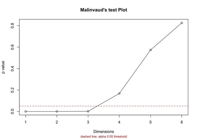
In our case, only the first three dimensions seems to be important since their p value is below 0.05, while the other three have a value equal to 0.167, 0.573 and 0.825 respectively.
Finally, as far as the greater-than-0.2 rule is concerned, the dimensions complying with that criterion can be located by inspecting the script’s textual output, which reports the list of dimensions with associated eigenvalues (after the ‘ca’ package). According to this rule, only the first dimension, accounting for more than half of the total inertia (i.e., 63.5%), should be retained.
The difference between the four methods underscoress the need to compare and find a balance between multiple dimension-retention criterions. In our case, a 2 or 3-dimensional solution seems appropriate.
Have you found this website helpful? Consider to leave a comment in this page.
