Seriation is an important method in archaeology. Simply put, 'seriation' is the relative ordering of things (e.g., graves, huts, rooms, coins, etc) according to combinations of traits. For example, graves can be ordered according to the various combinations of objects accompanying the dead. This rests on the assumption that artifacts (or any trait featuring past material cultures) appear, steadily increases in number, decrease, and then go out of fashion.
Various methods have been used in the history of archaeology to perform seriation, i.e. to sort the rows and columns of a contingency table in which, for example, graves (put in rows) are cross-tabulated against their content (i.e., artifacts; put in columns). Among these methods (comprising approaches as diverse as manual sorting and Multidimensional Scaling), Correspondence Analysis (CA) has been also used. Extensive treatment of the use of CA for seriation can be found in an interesting 1997 edited book (info here). Besides, CA keeps being used for seriation in very interesting recent monographs (link, link).
Recently, I came across the following interesting paper:
Halekoh, U., & Vach, W. (1999). Bayesian seriation as a tool in archaeology. In L. Dingwall, S. Exon, V. Gafney, S. Lafin, & M. van Leusen (Eds.), Archaeology in the Age of the Internet—CAA’97— Computer Applications and Quantitative Methods in Archaeology (Vol. 1997). Oxford: Archaeopress.
The paper interestingly proposes the use of Bayesian approaches to seriation problems.
What attracted my attention was the comparison between their Bayesian approach and CA. I do not want to dispute the proposed approach. I merely wish to stress that the criticism to CA, as to the claimed incapacity to detect the right chronological order in a particular case, should be downplayed.
The comparison between CA and the Bayesian seriation is built upon a fictional burials-related dataset, in which chronological and gender-related trends are intermixed. The dataset is reproduced below (left):
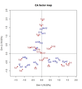
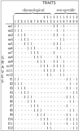 | Two remarks made by the Authors deserve some comment, in my opinion: 1) the fact that, in their opinion, for the given example correspondence analysis fails to detect the chronological order; 2) and that, as they stress, the first eigenvector puts the early male and female graves (m1-m4, f1-f4) just beside the late ones (m10-m12, f10-f12). On the contrary, I believe that CA is performing nearly as well as the Bayesian method discussed by the Author. As you can see from the plot of the CA dimension 1&2 (below left), there is no clear seriation structure (i.e., the so-called 'horseshoe effect'). Indeed, a roughly bell-shaped cloud of points is visible, and this should sound as a warning bell for the analyst since it could suggest (as, indeed, is the case) that different trends of variation are embedded in the data. This would therefore suggest to explore other dimensions as well, since as stressed in literature clear patterns suggesting a seriation can manifest on other CA sub-spaces. |
 | 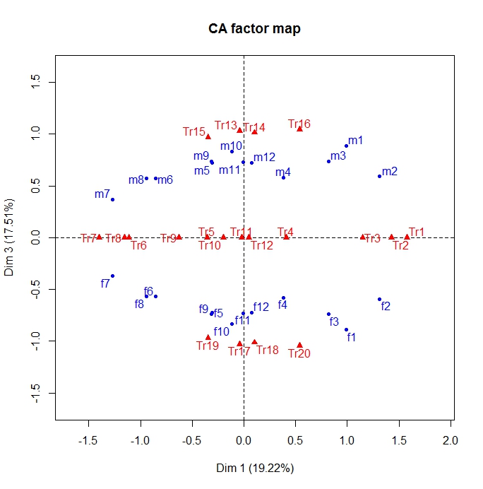 |
If one inspects the scatterplot for the CA dimensions 1&3 (above right) the picture begins to appear clearer. Indeed, CA is capturing the relative chronological order of the graves, albeit with some misplacements (on which I will return shortly). In fact, with reference to the 1 dimension, we can see that the grave number increases from right to left, both for male and female graves. Moreover, and interestingly, the third dimension (i.e., the vertical one) is capturing a trend of variation related to gender, separating male graves (in the upper quadrants of the scatterplot) from female graves (lower quadrants).
But there is more. If we take into account the 'traits' (burial goods), we can see that those ones being chronology-related are lined along the 1 dimension and, at the same time, they score zero on the third dimension. This means that those traits are not gender-related. Remarkably, the gender-related traits are correctly put at the opposite sides of the third (gender-related) dimension.
As for the aformentioned misplacements, let's take into account the group of male burials m1, m2, m3, m4, and m12, showing up in the upper-right quadrant of the scatteplot. Two things can be noted, which account for what could be wrongly considered a misplacement. Burial m1 is closer to m3 than to m2. This makes perfect sense. As a matter of fact, m1 has more traits in common with m3 (actually five trais: 2, 13, 14, and 16) than with m2 (four traits: 1, 2, 14, and 16). Secondly, m4 and m12 are close to one another because they do share trais 15 and 16, which are also shared by burial m10 and m11. For this very reason, the latter are not far (relatively speaking) from m4 and m12. Furthermore, burial m6 and m8 are close to one another since they feature two traits (14 and 15) that occur virtually in those two contexts alone. This also places these two burials far from the majority of the others. Finally, burial m7 is placed opposite the other burials since it contains just one sex-specific trait (13), which makes the burial stand out from all the other ones that feature 2-to-4 sex-specific traits.
A final note: as to the order of the graves in relation to the first dimension, the CA is NOT suggesting any absolute order. In other words, we cannot say that the 'true' order of the grave was actually from, say, m7 (oldest) to m2 (latest), or viceversa. The opposite could have been true. We can get from CA only a relative order, which can run either way. External chronological beacons are needed to convert the relative ordering into an absolute one.
Bottom line: CA allows to dissect different trends of variability that can be embedded in the data. Time is just one of such trends. In general, I believe that CA performs nearly as well as other approaches.
 RSS Feed
