'BRsim': R function for Brainerd-Robinson similarity coefficient (DOI: 10.13140/RG.2.1.2533.6080)
'BRsim' is an R function which allows to calculate the Brainerd-Robinson similarity coefficient. Information on this coefficient and on its computation can be found in the relevant literature (e.g., see Robinson's article available from on JSTOR). Even tough it has been devised many years ago, it keeps being used in archaeological literature as even a cursory search on Google plainly shows.
It is worth noting that a similar measure of similarity was independently devised in ecology-related research fields, and its first formulation traces back to a publication by Renkonen dating to 1938 (see Kohn-Riggs, Sample Size Dependence in Measures of Proportional Similarity, Marine Ecology Progress Series 9, 1982). In this field of study, the measure is termed measure of proportional similarity, and its independence from sample size is stressed. Further, Kohn and Riggs provide a substantive interpretation of this measure of similarity that it is worth keeping in mind: it measures the extent to which two samples are alike in composition, or the fraction of their totals in which they are alike in percentages of individuals of the various species.
Even though the calculations of the two similarity measures are slightly different, they are alike in their final outcome. Moreover, the former (in its original formulation) spans from 0 to 200, while the latter from 0.0 to 1.0.
The function provided here builds upon (and substantially expands) the one created by Daniel Weidele. Further, I thank Tyler Rinker for the help provided in fixing a critical bug in an earlier version of this function.
The function, whose code is provided below, takes as input a dataframe (i.e., a contingency table) in which the assemblages to be compared (e.g., tombs, huts, rooms, layers, etc) are in rows, while the variables featuring each assemblage (e.g., objects, pottery types, compositional groups, etc) are put in columns. The goal is to have a measure of how much similar each assemblage is to one another in terms of the proportions of the variables. See the Tab1 for a fictional example (dataset HERE).
|
The function is quite straightforward:
BRsim(x, correction, rescale) where x is the name of the dataset containing your data, which you have fed into R. The argument correction takes F if you do not want the coefficients to be corrected (I will elaborate on this later on), while T will provide corrected coefficients. The argument rescale takes F if you do NOT want the coefficient(s) to be rescaled between 0.0 and 1.0 (i.e., you will get the 'original' version of the Brainerd-Robinson coefficient (spanning from 0 [maximum dissimilarity] to 200 [maximum similarity]), while T will return rescaled coefficient(s). |

Tab1. Sample dataset
|
Suppose you gave your dataset the name 'mydata', the command to get the BR coefficient(s) (without corrections) would be:
BRsim(mydata, correction=F, rescale=T)
The command will report:
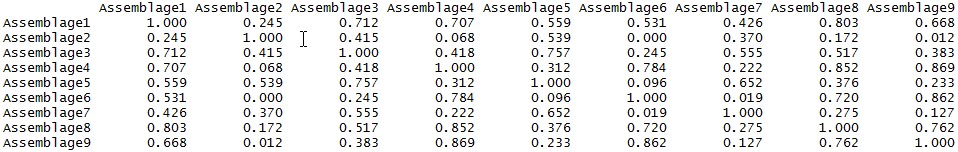
a) a correlation matrix in tabular form, displayed on the R console (see below);
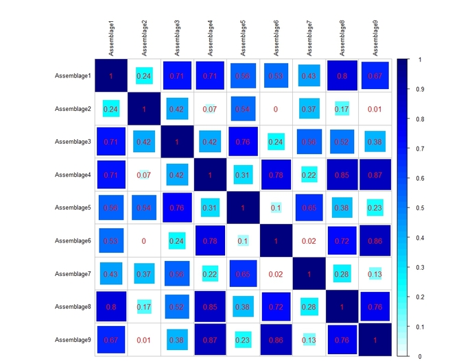
b) a heat-map representing, in a graphical form, the aforementioned correlation matrix (see below).
In the heat-map (which is built using the 'corrplot' package), the size and the color of the squares are proportional to the Brainerd-Robinson coefficients, which are also reported by numbers.
In this case, we will get rescaled coefficients.
If one is interested in assessing the statistical significance of the BR coefficient(s), an R script has been made available by Matthew A Peeples.
BRsim(mydata, correction=F, rescale=T)
The command will report:
a) a correlation matrix in tabular form, displayed on the R console (see below);
b) a heat-map representing, in a graphical form, the aforementioned correlation matrix (see below).
In the heat-map (which is built using the 'corrplot' package), the size and the color of the squares are proportional to the Brainerd-Robinson coefficients, which are also reported by numbers.
In this case, we will get rescaled coefficients.
If one is interested in assessing the statistical significance of the BR coefficient(s), an R script has been made available by Matthew A Peeples.
If you want the coefficient(s) to be corrected, the command is:
BRsim(mydata, correction=T, rescale=T)
Now, what this correction is?
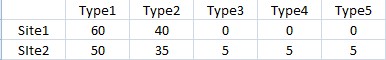
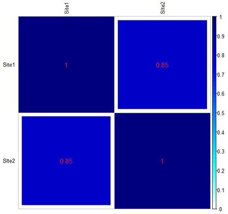
To put it in a nutshell, the correction is meant to account for the number of non-shared categories between assemblages. As becomes apparent reading the interesting article by C. H. McNutt (Seriation: Classical Problems and Multivariate Applications, in Southeastern Archaeology 24, 2, 2005), a rather high coefficient (namely, 170; equal to 0.85 on a scale from 0 to 1) may even arise when two assemblages have, for instance, just one or two categories in common (see tables below, reproducing Table 12 and 13 from McNutt's article).
BRsim(mydata, correction=T, rescale=T)
Now, what this correction is?
To put it in a nutshell, the correction is meant to account for the number of non-shared categories between assemblages. As becomes apparent reading the interesting article by C. H. McNutt (Seriation: Classical Problems and Multivariate Applications, in Southeastern Archaeology 24, 2, 2005), a rather high coefficient (namely, 170; equal to 0.85 on a scale from 0 to 1) may even arise when two assemblages have, for instance, just one or two categories in common (see tables below, reproducing Table 12 and 13 from McNutt's article).

Tab2
|
Tab3
|
As you can see from Tab2, the rather high BR similarity is essentially caused by the very similar frequency of Type 1 in both assemblages, which is the only type common to the two. The same applies to Tab3, where only two types are in common.
In order to "penalize" BR similarity coefficient(s) arising from assemblages with unshared categories, the function that I devised does what follows: it divides the BR coefficient(s) by the number of unshared categories plus 0.5. The latter addition is simply a means to be still able to penalize coefficient(s) arising from assemblages having just one unshared category. Also note that joint absences will have not weight on the penalization of the coefficient(s). It goes without saying that, in case of assemblages sharing all their categories, the corrected coefficient(s) turns out to be equal to the uncorrected one.
Below you can see the heat-maps deriving respectively from the two tables above, with uncorrected and corrected (rescaled) values:
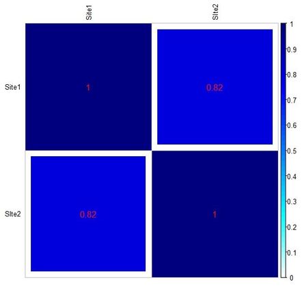
BR similarity coefficient, uncorrected (data from Tab2)
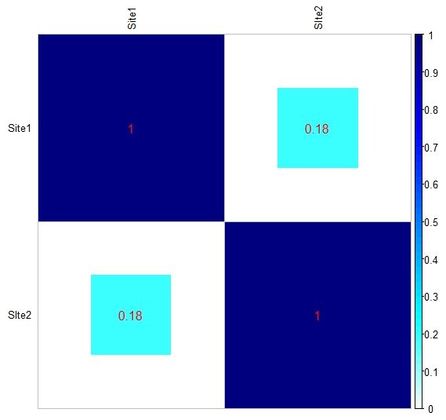
BR similarity coefficient, corrected (data from Tab2)
|
BR similarity coefficient, uncorrected (data from Tab3)
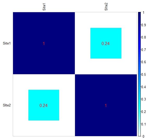
BR similarity coefficient, corrected (data from Tab3)
|
To load the function into R, just copy and paste the function below into the R console, and press return (or you can download the .R file HERE):
BRsim <- function(x, correction, rescale) {
  if(require(corrplot)){
    print("corrplot package already installed. Good!")
  } else {
    print("trying to install corrplot package...")
    install.packages("corrplot", dependencies=TRUE)
    suppressPackageStartupMessages(require(corrplot))
  }
  rd <- dim(x)[1]
  results <- matrix(0,rd,rd)
  if (correction == T){
    for (s1 in 1:rd) {
      for (s2 in 1:rd) {
        zero.categ.a <-length(which(x[s1,]==0))
        zero.categ.b <-length(which(x[s2,]==0))
        joint.absence <-sum(colSums(rbind(x[s1,], x[s2,])) == 0)
        if(zero.categ.a==zero.categ.b) {
          divisor.final <- 1
        } else {
          divisor.final <- max(zero.categ.a, zero.categ.b)-joint.absence+0.5
        }
        results[s1,s2] <- round((1 - (sum(abs(x[s1, ] / sum(x[s1,]) - x[s2, ] / sum(x[s2,]))))/2)/divisor.final, digits=3)
      }
    }
  } else {
    for (s1 in 1:rd) {
      for (s2 in 1:rd) {
        results[s1,s2] <- round(1 - (sum(abs(x[s1, ] / sum(x[s1,]) - x[s2, ] / sum(x[s2,]))))/2, digits=3)
      }
    }
  }
  rownames(results) <- rownames(x)
  colnames(results) <- rownames(x)
  col1 <- colorRampPalette(c("#7F0000", "red", "#FF7F00", "yellow", "white", "cyan", "#007FFF", "blue", "#00007F"))
  if (rescale == F) {
    upper <- 200
    results <- results * 200
  } else {
    upper <- 1.0
  }
  corrplot(results, method="square", addCoef.col="red", is.corr=FALSE, cl.lim = c(0, upper), col = col1(100), tl.col="black", tl.cex=0.8)
  return(results)
}
Final note:
in order for the function to produce the above chart, the 'corrplot' package must be installed in R. The function will automatically check if the package is already installed on your computer, otherwise it will attempt to install and load it.
in order for the function to produce the above chart, the 'corrplot' package must be installed in R. The function will automatically check if the package is already installed on your computer, otherwise it will attempt to install and load it.
Have you found this website helpful? Consider to leave a comment in this page.
