'chi.perm': R function for permutation-based Chi square test of independence (DOI: 10.13140/RG.2.1.3582.1846)
'chi.perm' is an R function which allows to perform the chi-square test of independence on the basis of permuted tables, whose number is selected by user. For the rationale of this approach, see for instance the nice description provided by Beh E.J., Lombardo R. 2014, Correspondence Analysis: Theory, Practice and New Strategies, Chichester, Wiley, at pages 62-64.
The function is quite straightforward:
chi.perm(data, B, resid, filter, thresh, cramer)
where:
data: is the dataframe containing the contingency table;
B: is the desired number of permutations (set at 1000 by default);
resid: takes TRUE or FALSE (default) if the user does or doesn't want to plot the table of Pearson's standardized residuals;
filter: takes TRUE or FALSE (default) if the user does or does't want to filter the Pearson's standardized residuals according to the threshold provided by the thresh parameter; by default, the threshold is set at 1.96, which corresponds to an alpha level of 0.05;
cramer: takes TRUE or FALSE (default) if the user does or doesn't want to calculate and plot the bootstrap confidence interval for Cramer's V.
Using for illustrative purposes the greenacre_data to which reference is made HERE, the figures 1 to 3 below are obtained by means of the following command:
chi.perm(greenacre_data, B=1000, resid=TRUE, filter=FALSE, cramer=TRUE)
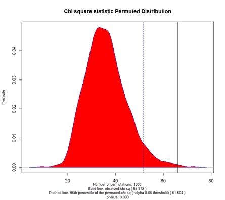
Fig. 1
|
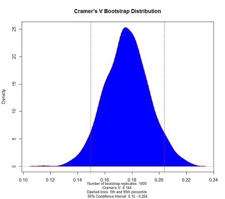
Fig. 2
|
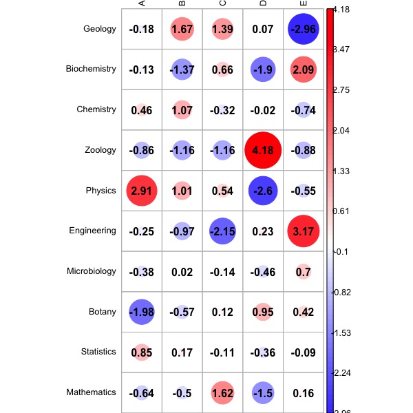
Fig. 3
|
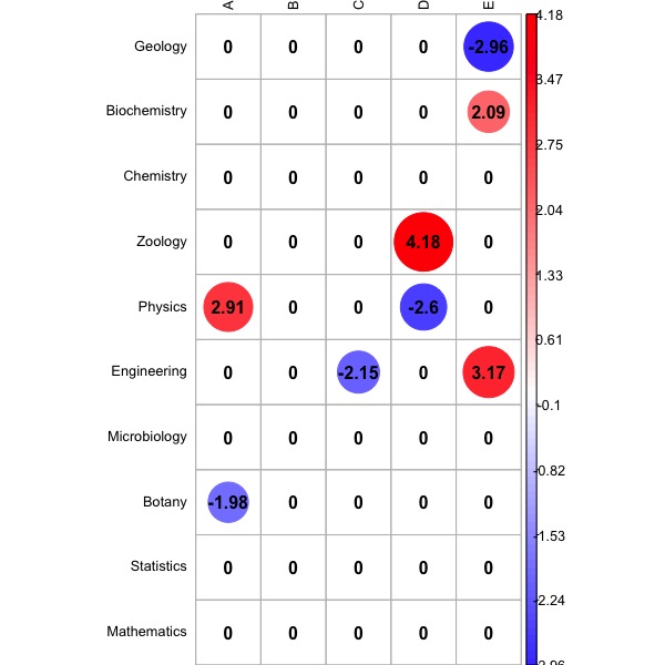
Fig. 4
|
Fig. 1 displays the permuted distribution of the chi square statistic based on 1000 permuted tables. The selected number of permuted tables, the observed chi square, the 95th percentile of the permuted distribution, and the associated p value are reported at the bottom of the chart.
Fig. 2 displays the bootstrap distribution of Cramer's V coefficient, based on a number of bootstrap replicates which is equal to the value of the function's parameter B. The 95% confidence interval for V is also reported. Fig. 3 displays the Pearson's Standardized Residuals: a colour scale allows to easily understand which residual is smaller (BLUE) or larger (RED) than expected under the hypothesis of independence.
Should the user want to only display residuals larger than a given threshold, it suffices to set the filter parameter to TRUE, and to specify the desidered threshold by means of the thresh parameter, which is set at 1.96 by default:
chi.perm(greenacre_data, B=1000, resid=TRUE, filter=TRUE, thresh=1.96, cramer=TRUE)
The output is displayed in Fig. 4 above.
The function requires the package 'corrplot', 'lrs', and 'InPosition' to be already loaded in R.
|
You can get the function via a small donation (about a couple of USD) -------------->
|
|
Upon making your donation, please do not forget to provide your preferred email contact where you will receive the file.
Have you found this website helpful? Consider to leave a comment in this page.
