'perm.t.test': R function for permutation-based t-test (DOI: 10.13140/RG.2.2.16735.46248 )
'perm.t.test' is an R function which allows to perform a permutation-based t-test to compare two independent groups. The test's results are graphically displayed within the returned chart. A permutation t-test proves useful when the assumption of 'regular' t-test are not met. In particular, when the two groups being compared show a very skewed distribution, and when the sample sizes are very unbalanced.
"The permutation test is useful even if we plan to use the two-sample t test. Rather than relying on Normal quantile plots of the two samples and the central limit theorem, we can directly check the Normality of the sampling distribution by looking at the permutation distribution. Permutation tests provide a “gold standard” for assessing two-sample t tests. If the two P-values differ considerably, it usually indicates that the conditions for the two-sample t don’t hold for these data. Because permutation tests give accurate P-values even when the sampling distribution is skewed, they are often used when accuracy is very important." (Moore, McCabe, Craig, Introduction to the Practice of Statistics, New York: W. H. Freeman and Company, 2009).
The function is straightforward:
perm.t.test(data, format, B)
where:
data: is the dataframe containing the data;
format: it takes long if the data are arranged in two columns, with the left-hand one containing the values, and the righ-hand one containing a grouping variable; it takes short if the values of the two groups being compared are stored in two different adjacent columns;
B: is the desired number of permutations (set at 1000 by default);
To illustrate the function, I will use the dataset Verizon that comes with the R package 'resample', and which is the same dataset used by Moore, McCabe and Craig in their book to illustrate the use of permutation t-test.
Once one has installed and loaded the 'resample' package, the dataset can be loaded by typing:
data("Verizon")
To put my function to work on the Verizon dataset, we can simply use:
perm.t.test(Verizon, format="long", B=10000)
The output chart is displayed below:
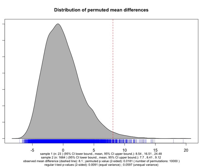
The chart diplays the distribution of the permuted mean difference between the two samples; a dashed line indicates the observed mean difference. A rug plot at the bottom of the density curve indicates the individual permuted mean differences.
Under the chart, a number of information are displayed. In particular, the observed mean difference, the number of permutations used, and the permuted p-value are reported. In the last row, the result of the regular t-test (both assuming and not assuming equal variances) is reported to allow users to compare the outcome of these different versions of the test.
It can be seen that, while the regular t-test (assuming unequal variance) does not point to a significant difference, the permutation t-test returns a significant p-value. As stressed by Moore, McCabe and Graig: "the strong skewness [of the permuted distribution of mean differences] implies that t-tests will be inaccurate". This accounts for the difference in p-value between the two versions of the test.
The function can be downloaded HERE (or copied/pasted from the code below). Finally, the function requires the package 'plyr' to be already loaded in R.
perm.t.test <- function (data,format,B=1000){
options(scipen=999)
if (format=="long") {
unstacked.data <- unstack(data) #requires 'plyr'
sample1 <- unstacked.data[[1]]
sample2 <- unstacked.data[[2]]
} else {
sample1 <- data[,1]
sample2 <- data[,2]
}
#get some statistics for the two samples
n1 <- length(sample1)
n2 <- length(sample2)
mean1 <- round(mean(sample1), 2)
mean2 <- round(mean(sample2),2)
error1 <- qnorm(0.975)*sd(sample1)/sqrt(n1)
error2 <- qnorm(0.975)*sd(sample2)/sqrt(n2)
sample1_lci <- round(mean1 - error1,2)
sample1_uci <- round(mean1 + error1,2)
sample2_lci <- round(mean2 - error2,2)
sample2_uci <- round(mean2 + error2,2)
#get regular t-test results (equal variance)
p.equal.var <- round(t.test(sample1, sample2, var.equal=TRUE)$p.value, 4)
#get regular t-test results (unequal variance)
p.unequal.var <- round(t.test(sample1, sample2, var.equal=FALSE)$p.value, 4)
#start permutation procedures
pooledData <- c(sample1, sample2)
size.sample1 <- length(sample1)
size.sample2 <- length(sample2)
size.pooled <- size.sample1+size.sample2
nIter <- B
meanDiff <- numeric(nIter+1)
meanDiff[1] <- round(mean1 - mean2, digits=2)
for(i in 2:length(meanDiff)){
index <- sample(1:size.pooled, size=size.sample1, replace=F)
sample1.perm <- pooledData[index]
sample2.perm <- pooledData[-index]
meanDiff[i] <- mean(sample1.perm) - mean(sample2.perm)
}
p.value <- round(mean(abs(meanDiff) >= abs(meanDiff[1])), digits=4)
plot(density(meanDiff), main="Distribution of permuted mean differences", xlab="", sub=paste("sample 1 (n:", n1,") (95% CI lower bound., mean, 95% CI upper bound.):", sample1_lci, ",", mean1, ",", sample1_uci, "\nsample 2 (n:", n2,") (95% CI lower bound., mean, 95% CI upper bound.):", sample2_lci, ",", mean2, ",", sample2_uci,"\nobserved mean difference (dashed line):", meanDiff[1],"; permuted p.value (2-sided):", p.value, "( number of permutations:", B,")\nregular t-test p-values (2-sided):", p.equal.var, "(equal variance) ;", p.unequal.var, "(unequal variance)"), cex.sub=0.78)
polygon(density(meanDiff), col="grey")
rug(meanDiff, col="blue")
abline(v=meanDiff[1], lty=2, col="red")
}
Have you found this website helpful? Consider to leave a comment in this page.
