'prob.phases.relat': posterior probability for different chronological relations between two Bayesian radiocarbon phases
(DOI: 10.13140/RG.2.1.3713.2560)
(DOI: 10.13140/RG.2.1.3713.2560)
'prob.phases.relat' is an R function which allows to calculate the posterior probability for different chronological relations between two phases defined via Bayesian radiocarbon modeling. Obviously, for the results to make sense, the phases have to be defined as independent if one wishes to assess what is the posterior probability for different relative chronological relations between them.
The rationale for this approach is made clear in this article by Buck et al 1992 (at pages 508-9), and it runs as follows: if we do not make any assumption about the relationship between the phases, can we test how likely they are to be in any given order?
Given two phases A and B, the function allows to calculate the posterior probability for:
A being within B
B being within A
A starting earlier but overlapping with B
B starting earlier but overlapping with A
A being entirely before B
B being entirely before A
sA being within B
eA being within B
sB being within A
eB being within A
where 's' and 'e' refer to the starting and ending boundaries of a phase.
Thanks are due to Dr. Andrew Millard (Durham University) for the help provided in working out the operations on probabilities.
|
The function, whose code is provided below, takes as input the table provided by the OxCal program as result of the Order query (see the pict to the right). Once the table as been saved from OxCal in .csv format (download a sample dataset here), you have to feed it in R by means of the following piece of code. Upon entering the command, a window will pop up allowing you to choose the .csv file.
mydata<-read.table(file.choose(), header=TRUE, sep=",", dec=".", as.is=T)
Make sure to insert the phases' parameters (i.e., the starting and ending boundaries of the two phases) in the OxCal's Order query in the following order: StartA, EndA, StartB, EndB. That is, first the start and end of your first phase, then the start and end of the second one. You can give any name to your phases, as long as the order is like the one described.
|
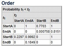
Output of the OxCal's Order query
|
Now, it is time to load the function into R. Just copy and paste the function below into the R console, and press return:
prob.phases.relat <- function(data) {
  if(require(Hmisc)){
    print("Hmisc package already installed. Good!")
  } else {
    print("trying to install Hmisc package...")
    install.packages("Hmisc", dependencies=TRUE)
    suppressPackageStartupMessages(require(Hmisc))
  }
  df <- as.data.frame(matrix(nrow = 10, ncol = 2))
  colnames(df)<-c("relation","posterior_prob")
  rel.labs <-c("A within B","B within A","A overlapping earlier than B","B overlapping earlier than A", "A entirely before B","B entirely before A", "sA within B", "eA within B", "sB within A", "eB within A")
  df[,1] <- rel.labs
  df[1,2] <- data[3,2]*data[2,5]
  df[2,2] <- data[1,4]*data[4,3]
  df[3,2] <- data[1,4]*data[3,3]*data[2,5]
  df[4,2] <- data[3,2]*data[1,5]*data[4,3]
  df[5,2] <- data[2,4]
  df[6,2] <- data[4,2]
  df[7,2] <- 1-(data[1,4]+(1-data[1,5]))
  df[8,2] <- 1-(data[2,4]+(1-data[2,5]))
  df[9,2] <- 1-(data[3,2]+(1-data[3,3]))
  df[10,2] <- 1-(data[4,2]+(1-data[4,3]))
  print(df)
  print(dotchart2(as.numeric(df$posterior_prob), labels=df$relation, sort=FALSE, lty=2, xlim=c(0.0, 1.0), xlab="posterior probability"))
}
After having fed into R the OxCal's table and my R function, you can simply run the function and sit back (hopefully) enjoying the results:
prob.phases.relat(mydata) where mydata is the name you gave to the table you fed into R.
prob.phases.relat(mydata) where mydata is the name you gave to the table you fed into R.
|
R will return a table (right) and a chart (below).
In our fictional example, there is 63% of posterior probability that phase A overlaps and is earlier than B. If we inspect the probability returned for the starting and ending boundaries, there is 81% probability that A ends within phase B, and 77% probability that B starts within A. This makes sense for phases which, as seen, are likely to be overlapping with one being earlier. |
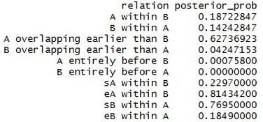
Table returned by the 'prob.phases.relat' function
|
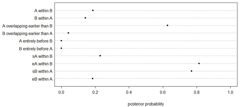
Dotplot returned by the 'prob.phases.relat' function
Final note:
in order for the function to produce the above chart, the 'Hmisc' package must be installed in R. The function will automatically check if the package is already installed on your computer, otherwise it will attempt to install and load it.
in order for the function to produce the above chart, the 'Hmisc' package must be installed in R. The function will automatically check if the package is already installed on your computer, otherwise it will attempt to install and load it.
Have you found this website helpful? Consider to leave a comment in this page.
