'plotJenks': R function for plotting univariate classification using Jenks' natural break method (DOI: 10.13140/RG.2.2.18011.05929)
'plotJenks' is an R function which allows to break a dataset down into a user-defined number of breaks and to nicely plot the results, adding a number of other relevant information. Implementing the Jenks' natural breaks method, it allows to find the best arrangement of values into different classes.
The function is quite straightforward:
plotJenks(data, n=3, brks.cex=0.70, top.margin=10, dist=5)
where
data: is a vector storing the data;
n: is the desired number of classes in which the dataset must be broken down (3 by default);
brks.cex: is used to adjust the size of the labels used in the returned plot to display the classes' break-points;
top.margin: is used to adjust the distance of the labels from the top margin of the returned chart;
dist: is used to adjust the distance of the labels from the dot used to display the data points.
To describe the use of the function, let's use a fictional dataset storing information about the wealth (in terms of the total cost of the accompayining burial items) of 78 graves in a cemetery. Let's assume the data are stored in a dataframe's column named $wealth. The dataframe name is mydata. Let's assume that we wish to break down the wealth values into 6 classes and we wish to work out the break-points that best capture "natural" groupings in the data.
We can put the function to work as follows:
plotJenks(mydata$wealth, n=6)
Note: all the other parameters are omitted, that is are left as they are by default.
The function returns the following chart:
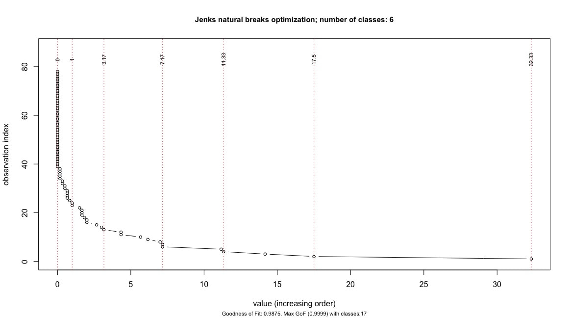
The wealth values are arranged on the x-axis in ascending order, while the index of the individual observations is reported on the y-axis. Vertical dotted red lines correspond to the optimal break-points which best divide the wealth values into the selected 6 classes. The break-points (and their values) are reported in the upper part of the chart, onto the corresponding break lines. Also, the chart's subtitle reports the Goodness of Fit value relative to the selected partition, and the partition which correspond to the maximum GoF value.
Finally, the function also returns some textual information which can be saved as follows:
res <- plotJenks(mydata$wealth, n=6)
that is storing them into an object to be further explored.
The user can access the information stored in the object res as follows:
- res$info: provide information about whether or not the method created non-unique breaks;
- res$classif: returns the created classes and the number of observations falling in each class;
- res$classif$brks: returns the classes' break-points;
- res$breaks$max.GoF: returns the number of classes at which the maximum GoF is achieved;
- res$class.data: returns a dataframe storing the values and the class in which each value actually falls into.
The function can be downloaded HERE. Alternatively, you can copy/paste the code below. Please note that the 'classInt' package must be already installed in R in order for the function to work properly.
plotJenks <- function(data, n=3, brks.cex=0.70, top.margin=10, dist=5){
df <- data.frame(sorted.values=sort(data, decreasing=TRUE))
Jclassif <- classIntervals(df$sorted.values, n, style = "jenks") #requires the 'classInt' package
test <- jenks.tests(Jclassif) #requires the 'classInt' package
df$class <- cut(df$sorted.values, unique(Jclassif$brks), labels=FALSE, include.lowest=TRUE) #the function unique() is used to remove non-unique breaks, should the latter be produced. This is done because the cut() function cannot break the values into classes if non-unique breaks are provided
if(length(Jclassif$brks)!=length(unique(Jclassif$brks))){
info <- ("The method has produced non-unique breaks, which have been removed. Please, check '...$classif$brks'")
} else {info <- ("The method did not produce non-unique breaks.")}
loop.res <- numeric(nrow(df))
i <- 1
repeat{
i <- i+1
loop.class <- classIntervals(df$sorted.values, i, style = "jenks")
loop.test <- jenks.tests(loop.class)
loop.res[i] <- loop.test[[2]]
if(loop.res[i]>0.9999){
break
}
}
max.GoF.brks <- which.max(loop.res)
plot(x=df$sorted.values, y=c(1:nrow(df)), type="b", main=paste0("Jenks natural breaks optimization; number of classes: ", n), sub=paste0("Goodness of Fit: ", round(test[[2]],4), ". Max GoF (", round(max(loop.res),4), ") with classes:", max.GoF.brks), ylim =c(0, nrow(df)+top.margin), cex=0.75, cex.main=0.95, cex.sub=0.7, ylab="observation index", xlab="value (increasing order)")
abline(v=Jclassif$brks, lty=3, col="red")
text(x=Jclassif$brks, y= max(nrow(df)) + dist, labels=sort(round(Jclassif$brks, 2)), cex=brks.cex, srt=90)
results <- list("info"=info, "classif" = Jclassif, "breaks.max.GoF"=max.GoF.brks, "class.data" = df)
return(results)
}
Have you found this website helpful? Consider to leave a comment in this page.
